Case Study 1: Idealized Flat-surface Uncoupled Model
The first case study presented here is an idealized uncoupled model with flat surface based on the first model presented by Munoz-esparza et al. [1]. The wind field is assumed to be uniform and constant throughout the simulation, and all the atmospheric options are turned off in this case. The main goal of this case is to introduce the very basics of WRF and WRF-Fire, and how to create an idealized model. As an uncoupled model, this case only represents Rothermel’s [2]rate of spread (ROS) theorem.
Input Files
In idealized cases, WRF-Fire requires three input files:
namelist.input: this file contains all of the WRF and WRF-Fire modelling parameters and assumptions
namelist.fire: fuel characteristics for different fuel types are defined in this file
Input_sounding: the atmospheric state including wind components along X and Y direction, temperature, and water vapor mixing ratio along the vertical axis is specified in this input file
Note
The input files are text files which can be generated/edited using text editors such as Notepad and Sublime Text.
Hint
The best way to generate the input files is to use sample inputs such as hill_simple and two_fires, and modify them as required.
Namelist.input
All the modelling parameters and assumptions for both WRF atmospheric model and WRF-Fire is defined in “namelist.input” file. This input file contains different sections controlling different aspects of the model such as control, domains setup, physics schemes, and fire module.
General Structure
The general structure of the “namelist.input” file is as follows.
&(section name)
.
.
.
(options within this section)
.
.
.
/
Note
comments can be defined using a “!”.
The options activated in each section for this case study are presented in this section.
&time_control
The temporal setup of the model, such as simulation duration, simulation date and time, and outputs interval, is controlled by this section. The options and values used for this case study is shown below.
&time_control
run_days                            = 0,
run_hours                           = 1,
run_minutes                         = 0,
run_seconds                         = 0,
start_year                          = 0001,
start_month                         = 01,
start_day                           = 01,
start_hour                          = 00,
start_minute                        = 00,
start_second                        = 00,
end_year                            = 0001,
end_month                           = 01,
end_day                             = 01,
end_hour                            = 1,
end_minute                          = 00,
end_second                          = 00,
history_interval_s                  = 120,
frames_per_outfile                  = 1,
restart                             = .false.,
!restart_interval                    = 30,
io_form_history                     = 2,
io_form_restart                     = 2,
io_form_input                       = 2,
io_form_boundary                    = 2,
/
Most of the options in this section are self-explanatory. In this case study, the model will be running for 1 hour (see options “run_days”, “run_hours”, etc.). The simulation start and end date and time are not important in most of the idealized cases, and therefore, the date is set to all 1 and the time is from 0 to 1 hour. Options “history_interval_s” and “frames_per_outfile” specify the output interval in seconds and the number of outputs per output file, respectively. For instance, these options are set to 120 and 1 in this case meaning WRF-Fire will generate outputs each 120 seconds and writes each output interval on a separate file. The options beginning with “io” defines the input/output file format, and option 2 used herein is for “NetCDF” format which is the typically used format in WRF and WRF-Fire.
&domains
This section controls domain setup of the model which includes number of domains, domains sizes, domains starting and ending points, grid size, and time step. The domain setup of this case is as follows.
&domains
time_step                           = 0,
time_step_fract_num                 = 1,
time_step_fract_den                 = 4,
max_dom                             = 1,
s_we                                = 1,
e_we                                = 51,
s_sn                                = 1,
e_sn                                = 51,
s_vert                              = 1,
e_vert                              = 101,
dx                                  = 100.00,
dy                                  = 100.00,
ztop                                = 2000,
grid_id                             = 1,
parent_id                           = 0,
i_parent_start                      = 0,
j_parent_start                      = 0,
parent_grid_ratio                   = 1,
parent_time_step_ratio              = 1,
sr_x                                = 4,
sr_y                                = 4,
/
“time_step” defines the model time step in seconds, and “time_step_fract_num” and “time_step_fract_den” specify the nominator and denominator of the fractional part of the time step in seconds, respectively. “max_dom” specifies the number of domains, and options starting with “s_” and “e_” are used to define the domain start and end point in west-east (we), south-north (sn), and vertical (vert) directions. Grid sizes in X and Y direction are defined using “dx” and “dy” in meters, and the model top is set to 2000 meters using “ztop” option. “grid_id” and “parent_id” options define the domain number and the its respective parent domain number. In this case, for instance, since the model only has one domain, the domain number is set to 1 and its parent number is 0 meaning that this is the outermost domain. “i_parent_start” and “j_parent_start” which specify the starting grid point of the domain within its parent domain are also set to zero in this case as it is a single domain model. “sr_x” and “sr_y” options defines the fire domain refining, and in this case, they are 4 resulting in a fire domain 4 times finer than the main atmospheric domain.
&physics
Physics section is used to activate physics schemes of WRF atmospheric model. Since in this case the goal is to represent Rothermel’s ROS equation, i.e., the model is uncoupled with uniform wind field, all the physics options are turned off as shown below.
&physics
mp_physics                          = 0,
ra_lw_physics                       = 0,
ra_sw_physics                       = 0,
sf_sfclay_physics                   = 0,
sf_surface_physics                  = 0,
bl_pbl_physics                      = 0,
bldt                                = 0,
cu_physics                          = 0,
cudt                                = 0,
isfflx                              = 0,
ifsnow                              = 0,
icloud                              = 0,
mp_zero_out                         = 0,
/
&dynamics
Dynamics section controls the parametrization schemes of WRF atmospheric model. This model uses WRF classic terrain-following vertical grid instead of a hybrid terrain-following and isobaric grid. This setup is indicated by turning off “hybrid_opt” option. The temporal discretization of the model is set to 3rd order Runge-Kutta scheme using “rk_ord” option which defines the order of the Runge-Kutta scheme. Diffusion options, “diff_opt” and “km_opt”, are turned off as we want to achieve a uniform constant wind field. Furthermore, surface drag and heat flux, “tke_drag_coefficient” and “tke_heat_flux”, are set to zero to create an idealized slip-free surface that will not affect the wind field. WRF atmospheric model of this case is ran non-hydrostatically by setting “non_hydrostatic” option to true. Horizontal momentum and scalar advection order is default 5, and vertical momentum and advection order is default 3. “time_step_sound” which defines the ratio of model time step to sounding time step is set to 20 in this case. Moisture and scalar advection, “moist_adv_opt” and “scalar_adv_opt”, are the default positive-definite scheme. The tracer option, “tracer_opt”, is set to 3 which is the value must be used for WRF-Fire simulations. This variable activates tracers in WRF atmospheric model to simulate smoke dispersion from fire.
&dynamics
hybrid_opt                          = 0,
rk_ord                              = 3,
diff_opt                            = 0,
km_opt                              = 0,
tke_drag_coefficient                = 0.0,
tke_heat_flux                       = 0.0,
non_hydrostatic                     = .true.,
h_mom_adv_order                     = 5,
v_mom_adv_order                     = 3,
h_sca_adv_order                     = 5,
v_sca_adv_order                     = 3,
time_step_sound                     = 20,
moist_adv_opt                       = 1,
scalar_adv_opt                      = 1,
tracer_opt                          = 3,
/
&bdy_control
This section specifies the atmospheric model’s boundary condition. Multiple options are available in idealized cases, and they are described in WRF Technical Note Chapter 6. For this case, the periodic boundary condition is activated.
&bdy_control
periodic_x                          = .true.,
symmetric_xs                        = .false.,
symmetric_xe                        = .false.,
open_xs                             = .false.,
open_xe                             = .false.,
periodic_y                          = .true.,
symmetric_ys                        = .false.,
symmetric_ye                        = .false.,
open_ys                             = .false.,
open_ye                             = .false.,
/
&namelist_quilt
The options within this section allow for reserving several CPU cores to manage output only. These options are useful when the domain is large, but in this simple case reserved CPU cores (“nio_tasks_per_group”) is set to zero.
&namelist_quilt
nio_tasks_per_group = 0,
nio_groups = 1,
/
&fire
To this point, all the previous sections were for setting up the WRF atmospheric model. This section includes the setting required for WRF-Fire fire spread platform. For the purpose of the tutorial, the options within “&fire” is divided into multiple sub-sections as follows.
ifire              = 2,
fire_fuel_read     = 0,
fire_fuel_cat      = 1,
“ifire” is used to activate or disactivate WRF-Fire. The available options are 0 and 2 which turns WRF-Fire off and on, respectively. By setting “fire_fuel_read” to 0, the model is configured to use a uniform fuel type defined by the user in “namelist.fire” file. Other choices for this option will be investigated in real data cases. “fire_fuel_cat” specifies the fuel category to be used in the simulation from “namelist.fire” input file. To illustrate, in this example, the fuel category is set to 1 meaning that WRF-Fire will use fuel category 1 from “namelist.fire” input file.
fire_num_ignitions     = 1,
fire_ignition_start_x1 = 1050.,
fire_ignition_start_y1 = 2000.,
fire_ignition_end_x1   = 1050.,
fire_ignition_end_y1   = 3000.,
fire_ignition_ros1 =   110,
fire_ignition_radius1  = 100,
fire_ignition_start_time1 = 10,
fire_ignition_end_time1  = 11,
The above set of options are used to define fire ignition characteristics. WRF-Fire supports for up to 5 ignition lines, and the number of ignition lines is defined using “fire_num_ignition” which is 1 in this case. The next four options specify the X and Y coordinates of ignition line start and end points in meters from the lower left corner of the domain. “fire_ignition_ros1” and “fire_ignition_radius1” specify the ignition line ROS during the ignition and ignition line radius, width in other words, respectively. The last two options define the ignition start and end time from the beginning of the simulation in seconds.
Note
The number 1 at the end of the above-mentioned ignition line characteristics indicates the ignition line number. Therefore, if 2 ignition lines are desired, all the above options must be repeated with the difference that the end number must be changed to 2. For instance, the ignition ROS of the ignition line 2 is “fire_ignition_ros2”.
Note
One of the known issues of WRF-Fire is that the fire does not ignite or ignites with a delay under special circumstances. In order to ensure fire ignition, the below equation must be satisfied: lfnnew=d -min(radius, ROS* (endts- timeign)<0; where d is the distance from ignition line to the nearest fire grid point, radius is ignition line radius, ROS is ignition rate of spread, and timeign and endts is ignition start and end time, respectively.
fire_print_msg     = 1,
fire_wind_height = 6.5,
fire_topo_from_atm = 1,
fire_atm_feedback = 0.0,
fire_viscosity = 0.4,
fire_upwinding = 7,
fire_boundary_guard=-1,
The first option, “fire_print_msg”, controls the output from WRF-Fire written on the standard output. Option 1 used in this case prints the basic information of fire module such as mean and maximum wind speed, area burned, and model time. “fire_wind_height” controls the height at which the wind components are calculated for Rothermel’s ROS equation which is typically 6.5 meters same as in this case. As mentioned earlier, this case is an uncoupled model meaning that the fire/atmosphere interaction is turned off. This is defined by “fire_atm_feedback” which is set to zero. “fire_viscosity” and “fire_upwinding” determine the artificial viscosity required for the level-set equation and the spatial discretization of the level-set differential equation, respectively. “fire_upwinding” 7 is for WENO5 scheme [3]. Lastly, the “fire_boundary_guard” specifies the number of cells from the domain boundary to stop the fire when it reaches that cell.
The “&fire” section of this case study is as follows.
&fire
ifire              = 2,
fire_fuel_read     = 0,
fire_fuel_cat      = 1,
fire_num_ignitions     = 1,
fire_ignition_start_x1 = 1050.,
fire_ignition_start_y1 = 2000.,
fire_ignition_end_x1   = 1050.,
fire_ignition_end_y1   = 3000.,
fire_ignition_ros1 =   110,
fire_ignition_radius1  = 100,
fire_ignition_start_time1 = 10,
fire_ignition_end_time1  = 11,
fire_print_msg     = 1,
fire_wind_height = 6.5,
fire_topo_from_atm = 1,
fire_atm_feedback = 0.0,
fire_viscosity = 0.4,
fire_upwinding = 7,
fire_boundary_guard=-1,
 /
Namelist.fire
The fuel characteristics required in Rothermel’s equation, such as fuel load, fuel height, surface area to volume ratio, and fuel moisture content, are specified in this file. Sample “namelist.fire” files provided with WRF-Fire (located at test/em_fire directory) are based on Anderson’s 13 fuel category [4], and they can be modified using a text editor. Moreover, the general structure of this file is same as the “namelist.input’ file. Available sections and options in this file are described in the rest of this section.
Note
same as “namelist.input”, modifying one of the sample files is highly recommended.
&fuel_scalars
This section includes the fuel characteristics that are constant among all the fuel types. “&fuel_scalars” parameters used for this case study is based on Rothermel’s model and Anderson’s 13 fuel categories, and they are as follows.
&fuel_scalars
cmbcnst  = 17.433e+06,
hfgl     = 17.e4 ,
fuelmc_g = 0.08,
fuelmc_c = 1.00,
nfuelcats = 13,
no_fuel_cat = 14
/
In the above parameters, the “cmbcnst” and “hfgl” parameters define combustion heat of dry fuel in J kg-1 and heat flux to ignite canopy in W m-2, respectively. The “fuelmc_g” and “fuelmc_c” specify the fuel moisture content of surface (ground) and canopy fuel, respectively. The total number of fuel categories are set to 13 using “nfuelcats” option, and non-burnable fuel is assigned fuel category 14 using “no_fuel_cat” option meaning that pixels defined with fuel category 14 will be considered as non-burnable, and they will not burn during the simulation.
&fuel_categories
Fuel characteristics for each fuel type are defined in this section. In the following “&fuel_categories” used for this case study, “windrf” is the wind adjustment factor which calculates the wind at mid-flame length from the wind speed at 6.5 meters. “fgi” and “fueldepthm” are used to specify the total fuel load in kg m-2 and fuel depth in meters for each fuel type, respectively. Fuel particle surface-area to volume ratio is defined in m-1 using “savr” parameter, and fuel moisture content of extinction is defined using “fuelmce” parameter. “fueldense” specifies the fuel particle density, which is 32 kg m-1 for solid and 19 kg m-1 for rotten fuels. “st” and “se” parameters specify fuel particle total and effective mineral content, respectively. “weight” parameter specifies the weighting factor used to calculate the heat flux from fire.
&fuel_categories
windrf= 0.36, 0.36, 0.44,  0.55,  0.42,  0.44,  0.44, 0.36, 0.36, 0.36,  0.36,  0.43,  0.46, 1e-7
fgi =  0.166, 0.897, 0.675, 2.468, 0.785, 1.345, 1.092, 1.121, 0.780, 2.694, 2.582, 7.749, 13.024, 1.e-7,
fueldepthm=0.305, 0.305, 0.762, 1.829, 0.61,  0.762, 0.762, 0.061, 0.061, 0.305, 0.305, 0.701, 0.914, 0.305,
savr = 3500., 2784., 1500., 1739., 1683., 1564., 1562., 1889., 2484., 1764., 1182., 1145., 1159., 3500.,
fuelmce = 0.12, 0.15, 0.25, 0.20, 0.20, 0.25, 0.40, 0.30, 0.25, 0.25, 0.15, 0.20, 0.25, 0.12,
fueldens = 32.,32.,32.,32.,32.,32.,32.,32.,32.,32.,32.,32.,32.,32.,
st = 0.0555, 0.0555, 0.0555, 0.0555, 0.0555, 0.0555, 0.0555, 0.0555, 0.0555, 0.0555, 0.0555, 0.0555, 0.0555, 0.0555,
se = 0.010, 0.010, 0.010, 0.010, 0.010, 0.010, 0.010, 0.010, 0.010, 0.010, 0.010, 0.010, 0.010, 0.010,
weight = 7.,  7.,  7., 180., 100., 100., 100., 900., 900., 900., 900., 900., 900., 7. ,
/
Input_sounding
The initial atmosphere state of the WRF atmospheric model is defined by “input_sounding” file. Same as other input files, this is also text file which can be edited using any text editors. The structure of “input_sounding” is as follows. The first row of the “input_sounding” determines the surface characteristics as demonstrated in the following table.
1,000.0 |
305.0 |
0.0 |
Surface pressure (pa) |
Surface temerature (K) |
Water vapor mixing ratio (kg kg-1) |
The other rows of the “input_sounding” file specify the atmosphere state at different elevations. The structure of these rows is demonstrated in the following table.
10.0 |
300.0 |
0.0 |
5.0 |
0.0 |
Elevation (m) |
Temerature (K) |
Water vapor mixing ratio (kg kg-1) |
Wind speed in X direction(m s-1) |
Wind speed in Y direction(m s-1) |
The complete “input_sounding” used for this study is as follows.
1000         305    0.0
1.00         300    0.0     5.0      0
6.00         300    0.0     5.0      0
9.10         300    0.0     5.0      0
18.3         300    0.0     5.0      0
18.35        300    0.0     5.0      0
91.2         300    0.0     5.0      0
100.         300    0.0     5.0      0
200.         300    0.0     5.0      0
300.         300    0.0     5.0      0
400.         300    0.0     5.0      0
500.         300    0.0     5.0      0
600.         300    0.0     5.0      0
700.         300    0.0     5.0      0
800.         300    0.0     5.0      0
900.         300    0.0     5.0      0
1000         300    0.0     5.0      0
1100         301    0.0     5.0      0
1200         302    0.0     5.0      0
1300         303    0.0     5.0      0
1400         304    0.0     5.0      0
1500         305    0.0     5.0      0
1600         306    0.0     5.0      0
1700         307    0.0     5.0      0
1800         308    0.0     5.0      0
1900         309    0.0     5.0      0
2000         310    0.0     5.0      0
2100         311    0.0     5.0      0
In this case study, the surface is assumed to be at 1,000 pa pressure level, and water vapor mixing ratio is assumed to be zero. The wind speed is uniform 5 m s-1 along the X direction. The surface temperature is set to 305 K. The temperature is assumed to be constant 300 K till 1 km altitude, and it increases linearly to 311 K from 1 to 2.1 km.
Note
The elevations specified in “input_sounding” do not need to match the WRF vertical levels. WRF interpolates the parameters from “input_sounding to model levels.
Sample Output
Sample outputs of this case study is shown in the below figures. These figures are generated using the in-house Python code to plot fire perimeter, topography, and wind field in idealized simulations. The mentioned Python code along with its description is available in this page. This model results are purely Rothermel’s ROS theorem as the fire/atmosphere coupling is turned off and the wind field is constant during the simulation. The “U” shape of the fire propagation, which is the well-known fire shape driven by wind, is clearly present in the results, and the fire is propagating along the wind direction indicating that the results are correct. Moreover, fire ROS is constant throughout the simulation, and it is equal to value resulted by Rothermel’s ROS equation for fuel type 1, short grass, under no topography and 5 ms-1 wind speed.
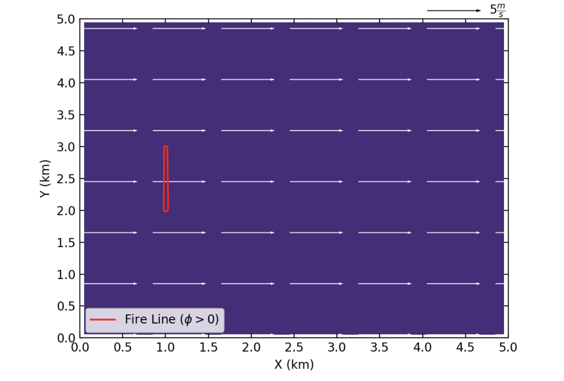
Beginning of the simulation
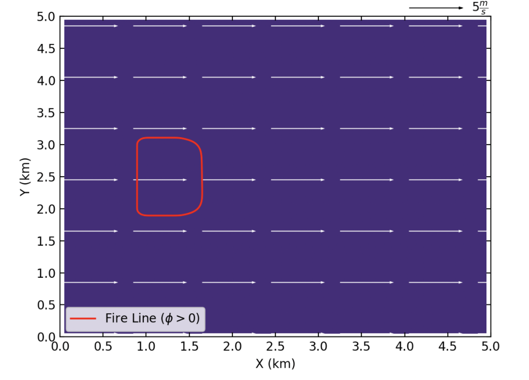
10 min after start of the simulation
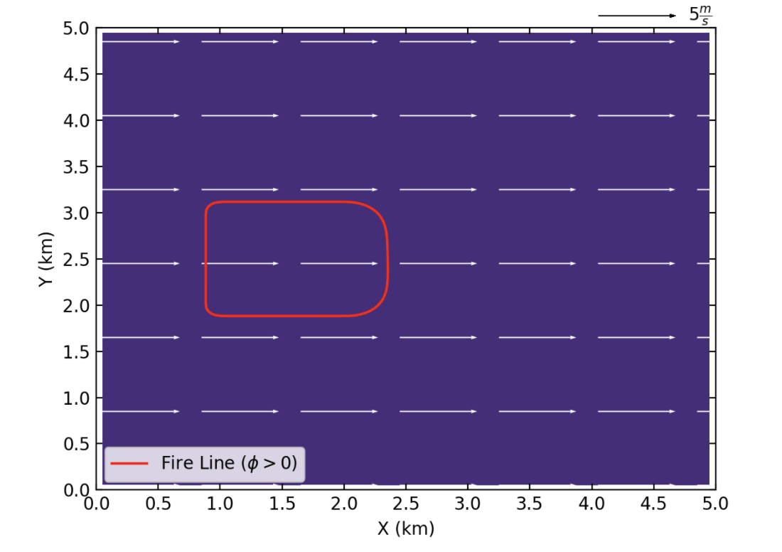
20 min after start of the simulation

End of the simulation
References
[1] D. Muñoz-Esparza, B. Kosović, P. A. Jiménez, and J. L. Coen, “An Accurate Fire-Spread Algorithm in the Weather Research and Forecasting Model Using the Level-Set Method,” J. Adv. Model. Earth Syst., vol. 10, no. 4, pp. 908–926, Apr. 2018, doi: 10.1002/2017MS001108.
[2] R. C. Rothermel, A mathematical model for predicting fire spread in wildland fuels. Intermountain Forest & Range Experiment Station, Forest Service, U.S. Dept. of Agriculture, 1972.
[3] P. A. Jiménez, D. Muñoz-Esparza, and B. Kosović, “A High Resolution Coupled Fire–Atmosphere Forecasting System to Minimize the Impacts of Wildland Fires: Applications to the Chimney Tops II Wildland Event,” Atmos. 2018, Vol. 9, Page 197, vol. 9, no. 5, p. 197, May 2018, doi: 10.3390/ATMOS9050197.
[4] H. E. Anderson, Aids to determining fuel models for estimating fire behavior, vol. 122. US Department of Agriculture, Forest Service, Intermountain Forest and Range …, 1981.